Industry Data Strategy
Demand Sensing for Consumer Goods Brands: The Data, the Measures and When It Pays
Demand sensing for consumer goods brands: the short-horizon signals it needs, forecast hierarchies, bias and WAPE, forecast value added, and when it pays.
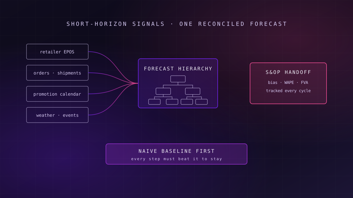
Demand sensing improves short-horizon forecasts for consumer goods brands by adding recent signals, such as retailer EPOS, orders, shipments, promotions and weather, to a statistical baseline. It pays where those signals arrive daily and decisions can still change. It needs a reconciled forecast hierarchy, honest bias and error measures, and proof each step beats a naive forecast.
Most demand planning teams already forecast. The question demand sensing answers is narrower: can the next one to six weeks be forecast better than the monthly plan allows, using data that arrives faster than the plan is refreshed? For a brand selling through grocers and convenience channels, the answer depends less on algorithms than on whether the right data arrives on time and in a shape the forecast can use.
Why Short-Horizon Forecasting Became a Data Problem
What this means for you: the gap between a monthly plan and weekly reality is where stock-outs and write-offs happen, and closing it is mostly a data-plumbing job.
Traditional demand planning works at monthly buckets, often at a brand or category level, and is refreshed once per sales and operations planning (S&OP) cycle. That is the right horizon for capacity and procurement decisions. It is the wrong horizon for deploying finished goods to distribution centres, allocating stock across retailers, or reacting to a promotion that is selling faster than planned.
Three things changed the economics. Retailers increasingly share daily or weekly point-of-sale data with suppliers. Order and shipment data now flows through integrated supply-chain systems rather than weekly extracts. And forecasting research has become far more practical, with large public benchmarks showing which methods hold up on real retail data.
The forecast that matters most for stock is the one the monthly plan is least able to produce.
The best known of those benchmarks is the M5 competition, run in 2020 on the sales history of a large US retailer. It asked entrants to forecast 42,840 hierarchical series, submitting 30,490 forecasts at product and store level that could be summed upwards. Its findings, published by Makridakis, Spiliotis and Assimakopoulos in the International Journal of Forecasting in 2022, are useful precisely because the data looks like a consumer goods brand's: intermittent, promotional and hierarchical. The revenue side of the same data, pricing and promotion return, is covered in our guide to revenue growth management analytics in CPG.
What Demand Sensing Actually Is
What this means for you: pin down the definition before buying a tool, because vendors use the term for very different things.
Demand sensing is short-horizon forecasting that updates frequently, typically daily or weekly, using the most recent demand signals to adjust a baseline forecast for the next few days or weeks. It sits underneath the S&OP demand plan, not in place of it. The demand plan answers how much will be sold next quarter; demand sensing answers where this week's and next week's stock should be.
It is distinct from three things it is often confused with. It is not demand shaping, which changes demand through price and promotion. It is not a replacement for consensus planning, which aligns commercial and supply views. And it is not simply a machine-learning forecast, because the gain comes as much from fresher inputs as from the model applied to them.
| Approach | Horizon and refresh | Main inputs | Choose it when |
|---|---|---|---|
| Monthly statistical plan | 3–18 months, monthly | Shipment or order history | Capacity, procurement and budget decisions dominate |
| Consensus demand plan | 1–18 months, monthly S&OP | Statistical plan plus sales and marketing input | Commercial events need agreement across teams |
| Demand sensing | 1–6 weeks, daily or weekly | EPOS, orders, shipments, promotions, weather, events | Deployment and allocation decisions can still change |
| Promotion forecasting | Event-specific | Promotion history, mechanics, display and feature | Promotions drive a large share of volume |
The Short-Horizon Signals and What Each Needs
What this means for you: each signal brings its own delay, grain and quality problem, and the forecast inherits all of them.
Retailer EPOS
Point-of-sale data is the closest signal to consumer demand. It arrives at store and product level from the retailers that share it, on their schedule and in their product hierarchy. The work is mapping retailer product codes to your own, handling store openings and closures, and detecting gaps where a store's feed silently stopped. EPOS also shows sales, not demand: when a shelf is empty, sales fall to zero while demand does not.
Orders and Shipments
Orders show what retailers intend to buy; shipments show what you actually delivered. Both are internal and timely, but both carry retailer behaviour on top of consumer demand: forward buying ahead of price increases, order batching, and cuts when supply is short. A forecast trained on shipments alone learns your past supply constraints as if they were demand.
Promotions, Weather and Events
The promotion calendar must be the agreed one, with mechanics, depth, dates and retailer, kept in a structured form rather than in slide decks. Weather matters for categories such as drinks, ice cream and seasonal goods, and barely at all for others. Events, from bank holidays to major sporting fixtures, need a maintained calendar with regional detail.
Failure mode
Failure mode: training on constrained history
If past shipments were cut because stock ran out, a model learns that demand was lower than it was. Flag constrained periods in the history, or use EPOS and order data to reconstruct unconstrained demand, before training anything.
Feeding these signals reliably is ordinary data engineering for frequently refreshed sources, and the patterns for picking up changes in source systems without full reloads are set out in our guide to change data capture.
Forecast Hierarchy and Reconciliation
What this means for you: forecasts made at different levels will disagree, and someone has to decide which one wins before supply acts on them.
Consumer goods forecasts live in a hierarchy: product, brand and category on one axis; store, retailer, region and distribution centre on another; days, weeks and months on a third. A forecast made at product-store level will not sum to the forecast made at brand-region level, because each was fitted to different noise.
Reconciliation is the step that makes them consistent. Bottom-up summing preserves detail but carries noise upwards. Top-down allocation is stable but loses local patterns. Optimal reconciliation methods, which combine forecasts from every level, have become standard practice in forecasting research and were used widely in M5. The method matters less than the rule: one reconciled set of numbers, at every level, before anyone plans against them.
Key idea
Agree the planning grain before the model
Decide the level at which each decision is made: deployment by product and distribution centre, allocation by product and retailer, production by product family. Forecast at the level the decision needs, and reconcile everything else to it.
The hierarchy itself is master data. Product, customer and location hierarchies that match how retailers sell are the same foundation RGM depends on, and a pre-built consumer goods data template can shorten that work. When to start from a template and when to build from scratch is set out in our guide to industry data templates.
Measuring Forecasts Honestly: Bias, WAPE, MAPE and FVA
What this means for you: a single accuracy number hides the two failures that cost money, which are persistent bias and the steps that make the forecast worse.
Bias Before Accuracy
Bias is the tendency to forecast consistently high or low. It is the measure that maps most directly to cost: persistent over-forecasting builds stock and write-offs, persistent under-forecasting causes lost sales. Track it by product tier and horizon, and treat a bias that persists across several cycles as a process problem rather than noise.
WAPE and MAPE
Mean absolute percentage error (MAPE) averages the percentage error of each item. It is easy to explain but distorted by low-volume items, where a small absolute miss becomes a huge percentage. Weighted absolute percentage error (WAPE) divides total absolute error by total actual volume, so it reflects where the volume is. For a range with a long tail of slow sellers, WAPE is usually the more decision-useful headline, with MAPE kept for item-level diagnosis.
A forecast step that cannot beat a naive forecast is not a refinement. It is a cost.
Forecast Value Added
Forecast value added (FVA), framed by Michael Gilliland in 2002, measures the change in forecast error contributed by each step in the process, starting from a naive forecast such as "next week equals last week". The statistical model, the demand-sensing adjustment, the sales override and the consensus meeting are each measured against the step before. Any step that does not improve the result is, in Gilliland's framing, process waste.
Research on judgemental adjustments supports the point. Fildes, Goodwin, Lawrence and Nikolopoulos, in the International Journal of Forecasting in 2009, found across supply-chain companies that small adjustments added little and that optimistic upward adjustments often made forecasts worse. A later pooled analysis by Fildes, Goodwin and De Baets found adjustments improved accuracy and bias for only around half of the products studied.
Readiness signal
Readiness signal: can you show FVA by step?
If you cannot show, for last quarter, whether the sales override improved or worsened the statistical forecast, start there. It costs little, needs no new tooling, and usually identifies effort that can stop immediately.
Where Machine Learning Helps, and Where Baselines Win
What this means for you: match the method to the volume and pattern of each product, rather than applying one model to the whole range.
Machine learning earns its place where there are many related series, rich explanatory data and enough history. Gradient-boosted tree models were widely used among the strongest M5 entries, largely because one model can learn across thousands of related products and absorb promotions, prices and calendar effects together. For high-volume, promoted products with good EPOS coverage, that is a real advantage.
Statistical baselines still win in several places. New products have no history to learn from. Slow sellers with intermittent demand are dominated by noise, where simple methods designed for intermittent series are hard to beat. And for stable, unpromoted lines, exponential smoothing is cheap, explainable and often as accurate. Keeping models in production also has a cost, set out in our guide to running predictive models in production.
High-volume, promoted
Machine learning across related products, with promotions, prices and EPOS as features. This is where demand sensing pays most.
Stable, unpromoted
Exponential smoothing or a similar statistical baseline. Cheap, explainable, and often as accurate.
Slow and intermittent
Methods built for intermittent demand, with stock policy doing more of the work than the forecast.
Whichever method is used, predictive models built for production need the same discipline: a naive baseline, a holdout period, and error tracked after go-live rather than only in the pilot.
The Handoff to Sales and Operations Planning
What this means for you: a short-horizon forecast that does not change a decision is a dashboard, not a capability.
Demand sensing feeds a small number of operational decisions: deploying stock from factories to distribution centres, allocating constrained stock across retailers, and adjusting short-term production. Each needs a named owner, a decision cadence and a rule for when the sensed forecast overrides the plan.
The S&OP process stays in charge of the medium term. Where the sensed forecast drifts persistently from the consensus plan, that drift is an input to the next S&OP cycle, not a reason to re-plan every week. Teams that let both forecasts drive the same decision end up with two numbers and no accountability.
The definitions behind those numbers, such as what counts as a sale, a return, or a promotional week, belong in a shared semantic layer so planning, sales and finance read the same figures.
When Demand Sensing Is Not Worth It
What this means for you: for some brands, better master data and a disciplined monthly process will deliver more than any sensing tool.
Demand sensing is the wrong investment when retailers do not share timely sell-out data and most volume flows through channels with no EPOS visibility. It adds little where supply cannot respond inside the sensing horizon: if production is locked six weeks out and stock cannot be moved between depots, a better forecast for next week changes nothing.
It is also premature when the basics are missing. If product hierarchies do not match retailers, constrained periods are not flagged, and nobody measures bias or FVA, the first gains come from fixing those, and a sensing layer built on top inherits every flaw. For many mid-sized brands, the higher-return work is in the commercial analytics covered by our guide to retail big data use cases that pay back.
Where to Start: A Ten-Week Forecast Value Review
What this means for you: measure before you buy, and let the numbers decide where demand sensing goes first.
Baseline and segment
Build a naive forecast, segment the range by volume and variability, and measure bias and WAPE by segment and horizon for the last year.
Measure FVA by step
Compare each process step with the one before it: statistical model, overrides, consensus. Identify steps that add error.
Pilot one decision
Add EPOS and orders for one segment and one decision, such as deployment for high-volume promoted lines, and measure the change against the baseline.
The scope is deliberately narrow: ten weeks covers a measured pilot on one segment and one decision, not a rollout across the range. The output is a written case for where demand sensing would pay, where it would not, and which process steps can stop. That case, and the analytics and reporting that tracks it afterwards, is what justifies the next investment.
Frequently Asked Questions
What is demand sensing in consumer goods?
Demand sensing is short-horizon forecasting, usually for the next one to six weeks, that updates daily or weekly using recent signals such as retailer point-of-sale data, orders, shipments, promotions and weather. It adjusts a statistical baseline for operational decisions like stock deployment and allocation, and sits underneath the monthly sales and operations plan rather than replacing it.
What data does demand sensing need?
It needs recent sell-out data from retailer point-of-sale feeds where available, orders and shipments, an agreed promotion calendar, weather and event calendars for sensitive categories, and product, customer and location hierarchies that match how retailers sell. History must also flag periods when supply was constrained, so models do not mistake stock-outs for low demand.
Should we measure forecasts with MAPE or WAPE?
Use both, for different jobs. WAPE divides total absolute error by total volume, so it reflects where volume sits and suits headline reporting for ranges with many slow sellers. MAPE averages item-level percentage errors and is distorted by low-volume items, but remains useful for diagnosing individual products. Track bias alongside both, because persistent bias drives stock cost.
What is forecast value added?
Forecast value added measures how much each step in a forecasting process improves or worsens accuracy compared with the step before, starting from a simple naive forecast. It shows whether statistical models, manual overrides and consensus meetings are adding value. Steps that consistently make the forecast worse can be stopped, which often saves effort before any new tooling is bought.
When is demand sensing not worth the investment?
It rarely pays when retailers do not share timely sell-out data, when supply cannot respond within the sensing horizon, or when basics are missing, such as matched product hierarchies, flagged stock-outs and measured bias. In those cases, fixing master data and measuring forecast value added in the existing process usually delivers more than a sensing tool.
Unolabs is a Data and AI first engineering consultancy, headquartered in the United Kingdom with engineering operations in Pune and active engagements across the UK, Australia, and Hong Kong. We help enterprises build the architectural foundation for autonomous AI execution — governed data platforms, semantic intelligence, and agentic systems that enterprises can stand behind.
If you are weighing whether demand sensing would pay for your range, book a discovery call and we will work through it with you.
More Where
This Came From.
New architectural deep-dives land every two weeks. Pick your channels and we will send them as they publish.
Continue reading
- Industry Data StrategyRevenue Growth Management Analytics in CPG: The Data Foundations It NeedsWhat revenue growth management analytics in CPG needs: price-pack data, promotion effectiveness, EPOS and syndicated feeds, and trade spend finance trusts.13 min read
- AI Readiness & StrategyThe Agent Tax: Why Replacing Your RPA Bots with AI Agents Could Blow Up Your Automation BudgetSwapping RPA bots for AI agents turns a fixed automation cost into one that scales with volume. The four cost lines most business cases leave out.15 min read
- Agentic ArchitecturesDesigning Production Agentic AI Systems: Architecture Patterns, Guardrails, and EvaluationHow production agentic AI is built: the agent loop, typed tool contracts, guardrail config, evaluation harnesses, and the gates that grant autonomy safely.18 min read
See whether demand sensing would pay for your range
We will measure your current forecast against a naive baseline by product tier and horizon, and show where short-horizon signals would add value and where they would add noise.
Book a Forecast Value Review